These instructions are applicable to various versions, including Excel Office 365, 2021, 2019, 2016, 2013, 2010, and 2007, as well as Excel Online and Excel for Mac 2016 and later.
Have you ever struggled with scrolling through a large spreadsheet and losing sight of your headers or important data? If so, you’re not alone. Many Excel users face this problem when working with big datasets that span across multiple rows and columns.
Fortunately, there is a simple solution to this problem: freezing rows and columns in Excel. By freezing rows and columns, you can lock them in place so that they remain visible no matter how far you scroll down or across your spreadsheet. This way, you can easily keep track of your data and avoid confusion or errors.
In this article, we’ll show you how to freeze rows and columns in Excel with easy-to-follow steps and examples. Let’s get started.
What is the “Freeze Panes” function and what can it do?
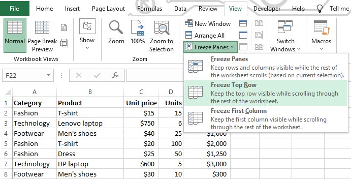
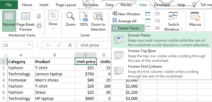
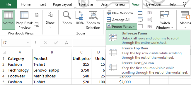
The “Freeze Panes” feature allows you to freeze rows and columns in Excel. You can find it in the View tab on the top ribbon under the Window group with three options.
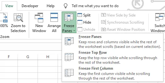
- Freeze Panes: This option allows you to freeze any row or column you want by selecting the cell that is below the last row and to the right of the last column you want to freeze. For example, if you want to freeze rows 1 and 2 and column A, select cell B3 and then click on Freeze Panes.
- Freeze Top Row: This option lets you freeze the top row of your spreadsheet (row 1) without selecting any cell. This is a shortcut that saves you time and effort if you want to freeze the top row only.
- Freeze First Column: This option lets you freeze the first column of your spreadsheet (column A) without selecting any cell. This is another shortcut that saves you time and effort if you want to freeze the first column only.
As you can see, Freeze Panes features allow you to lock a row or a column in place so that it remains visible when you scroll through your spreadsheet. This can help you keep track of your headers, labels, or categories while working with large datasets.
How to Freeze a Row in Excel
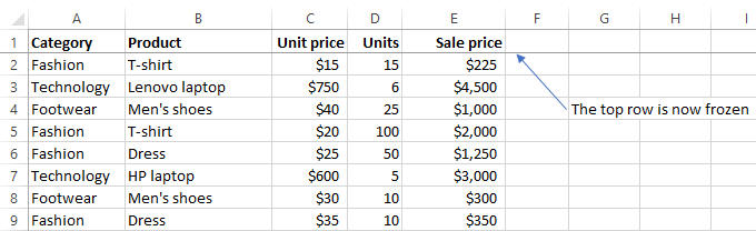
One of the most common and shortcut ways to freeze a row (1) without selecting any cell in the spreadsheet is to the Freeze Top Row when you have a header row that contains important information about your data, such as column names, titles, or labels.
By freezing the top row, you can keep these headers visible while scrolling down your data.
To freeze the top row in Excel, follow these steps:
- Open your Excel spreadsheet and ensure the first row contains the headers or labels you want to freeze.
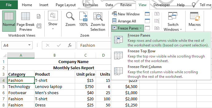
- Go to the View tab, and under the window group click on Freeze Panes > Freeze Top Row.
You will see a darker line below the first row, indicating that it is frozen. You can now scroll down your data and see that the first row remains on the screen.
How to Freeze Multiple Rows in Excel
If your header or label isn’t limited to just the top row, and you want to freeze multiple rows with headings, follow these steps:
- Select the first cell in the row just below the last row you want to freeze or the entire row.
For example, if you want to freeze row 3, you need to select cell A4 or the entire row 4. Then, - Go to the View tab, and under the window group click on Freeze Panes > Freeze Panes.
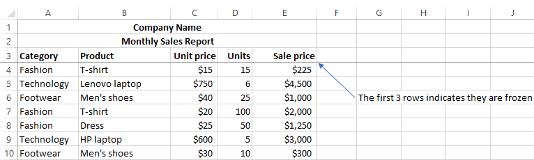
A darker line below the first 3 rows indicates they are frozen as you scroll down, keeping them on the screen.
How to Freeze a Column in Excel
You may have a column of category names on your dataset that you want to keep locked while moving to right your data.
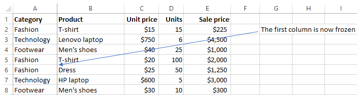
In this case, you can use the Freeze First Column option. It is another shortcut way to lock the first column (A) of your spreadsheet without selecting any cell.
- Open your Excel spreadsheet.
- Go to the View tab, and under the window group click on Freeze Panes > Freeze First Column.
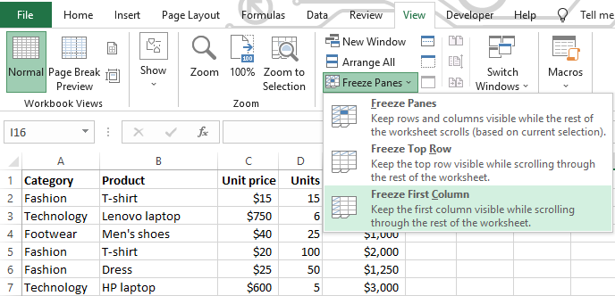
A darker line to the right of the Freeze First Column shows it’s frozen. As you scroll right, it stays on the screen.
How to Freeze Multiple Columns in Excel
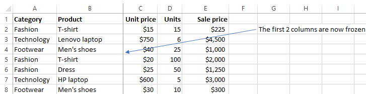
To freeze multiple columns with categories when your selection isn’t restricted to just the first column, follow these steps:
- Select the first cell in the column to the right of the last column you want to freeze or the entire column.
For example, if you want to freeze column 2, you need to select cell C1 or the entire column 3. Then, - Go to the View tab, and under the window group click on Freeze Panes > Freeze Panes.
The first 2 columns will have a darker line on their right side, which means they are frozen. You can scroll to the right and see that the first 2 columns don’t move from the screen.
How to Freeze Rows and Columns in Excel
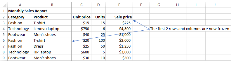
You may have an Excel dataset with two rows of headers and two columns of category names that you want to keep visible while scrolling across your data. In this case, you want to freeze rows and columns at the same time. then, follow these steps:
- Select the cell that is at the intersection of the rows and columns that you want to freeze.
For example, if you want to freeze the first 2 rows and the first 2 columns, you need to select cell C3. - Go to the View tab, and under the window group click on Freeze Panes > Freeze Panes.
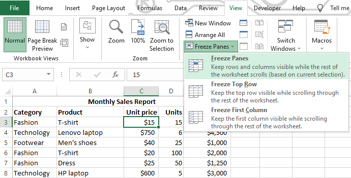
No matter how you scroll, you can always see the header rows and leftmost columns of your spreadsheet. They have darker lines to stand out.
How to Unfreeze Rows and Columns in Excel
If you want to unfreeze rows or columns and return to normal viewing in your spreadsheet, then.
Go to the View tab, and under the window group click on Freeze Panes > Unfreeze Panes.
You can scroll through your spreadsheet normally without any rows and columns staying in place.
How to Freeze Rows and Columns in Excel on Mac
If you’re using Excel on Mac, you can also freeze rows and columns in your spreadsheet using a similar process as Windows users.
- Select the cell that is below the last row and to the right of the last column that you want to freeze.
For example, if you want to freeze rows 1 and 2 and column A, select cell B3. - Go to the View tab, and under the window group click on Freeze Panes > Freeze Panes.
That’s how you can freeze rows in Excel for Mac. If you want to unfreeze them, go back to the View tab, click on Freeze Panes, and select Unfreeze Panes.
Note: If you’re using an older version of Excel for Mac, such as 2013, 2011, or 2008, you may not have a View tab on your ribbon. In this case, you can access the Freeze Panes feature from the Layout tab on your menu bar.
How to Freeze Rows and Columns in Google Sheets
If you’re using Google Sheets instead of Excel, you can also freeze rows and columns in your Google Sheets using an almost similar feature. To freeze rows and columns follow these steps:
- Freeze Rows: Select the row or any cell in the row you want to freeze. Then, Go to the View tab > Freeze > Up to row (X).
- Freeze Columns: Select the column or any cell in the column you want to freeze. Then, Go to the View tab > Freeze > Up to column (X).
- Unfreeze Rows and Columns: Go to the View tab > Freeze > No rows/No columns.
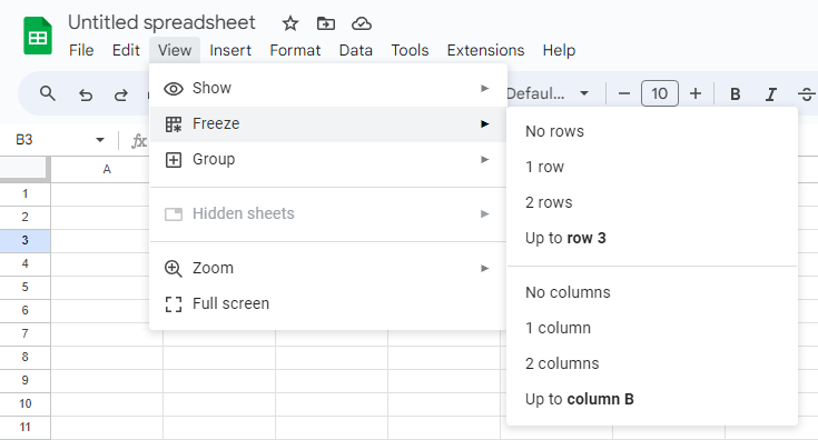
If you want to freeze just 1 and 2 no rows and columns, you don’t need to select any row or column. Go to the View > Freeze > & select 1 or 2 rows/columns you want to freeze.
You will see a darker line below and right of the frozen area, indicating that it is locked in place. You can now scroll down and right your data and see that the frozen row(s) and column(s) remain on the screen.
Conclusion
Freezing rows and columns in Excel is a useful technique that can help you work with large datasets more effectively and efficiently.
We hope we’ve shown you how to freeze rows and columns in Excel for Windows, Mac, and Google Sheets with clear instructions and examples.
Try it out for yourself and see how it works for your needs.
Please share it with your friends or colleagues who might find it useful.
Thank you for reading!