Pareto chart in Excel: how to create it

How to create a Pareto chart in Excel? Do you want to know the major causes on which you should devote your efforts? Here is the reason why you should read this article. In this article, I will show you how to make a Pareto chart in Excel.

A Pareto chart is a kind of chart that includes both bars and a line graph, with the bars representing individual values in descending order and the line representing the cumulative total.

Why create a Pareto chart?

Vilfredo Pareto was an Italian economist. From him derives a famous principle from which the relative Pareto analysis derives.

The principle states that about 80% of the effects come from 20% of the causes. For this reason, the Pareto principle is sometimes called the 80/20 rule.

This principle has several practical applications in different sectors.

Here are some examples of the Pareto principle that can be found in real life.

• 20% of the bugs often cause 80% of errors and crashes in the software.
• In economics, 20% of the richest countries have around 80% of the world‘s income.
• 80% of complaints come from 20% of customers.
• 20% of sellers make 80% of sales.

Creating the Pareto chart is essential, as it allows you to identify the most significant factors to focus on.

In this article, we are going to show you how to create a Pareto chart in Excel.

How to create a Pareto chart in Excel

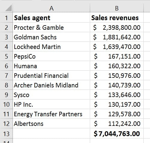
Let’s start with the analysis of a practical case.

In this example, we see that around 80% of sales come from 20% of sellers.

The Pareto chart, also called the Pareto analysis, is a chart that is based on a relative on principle.

In Excel, it is an ordered column chart that contains both vertical bars and a horizontal line.

The bars in the Histogram represent the relative frequency of the values. They are in descending order.

The line represents the cumulative total percentage.

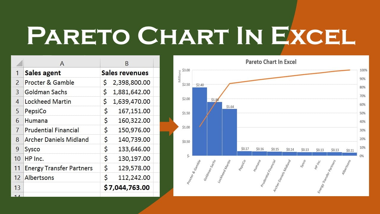
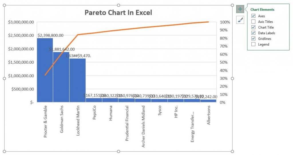
Here is an example of a typical Excel Pareto chart.

As you can see, the Pareto chart highlights the main elements within a data range. It shows the relative importance of each component over the total.

Creating a Pareto chart in Excel is easy. The Pareto chart is a type of built-in chart.

Follow these simple steps to create it.

Select the data range. Alternatively, just select one cell – Excel will select the rest.

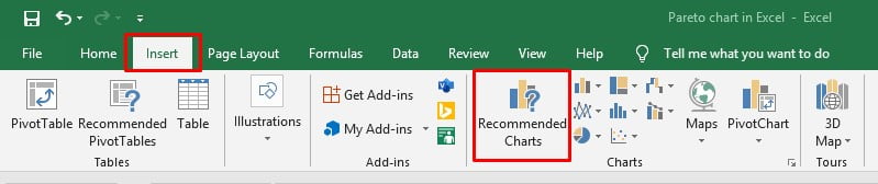
Click the Recommended Graphics command in the Graphics group of the Insert tab.

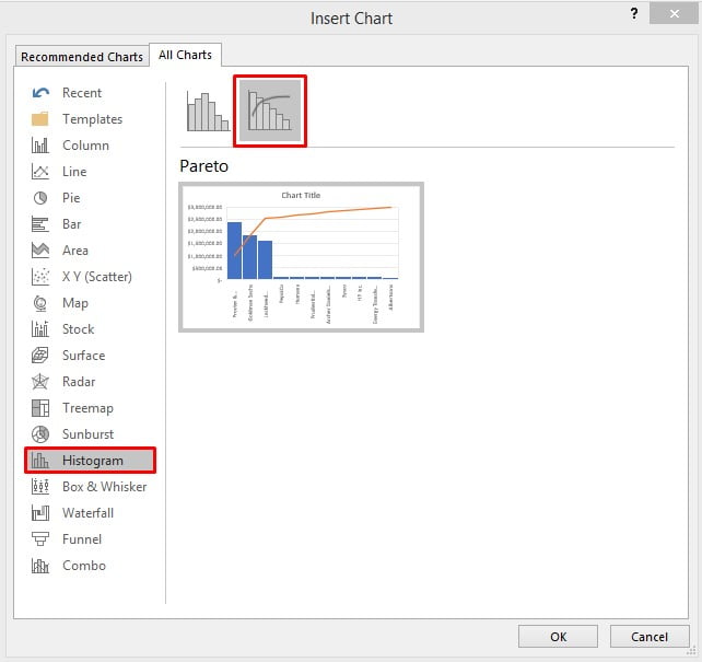
Click on the All Charts tab in the Insert Chart dialog box.

Select the Histogram in the left pane.

Click on the Pareto thumbnail.

Finally, click the OK button.

Alternatively, click on the Recommended Charts tab in the Insert Chart dialog.

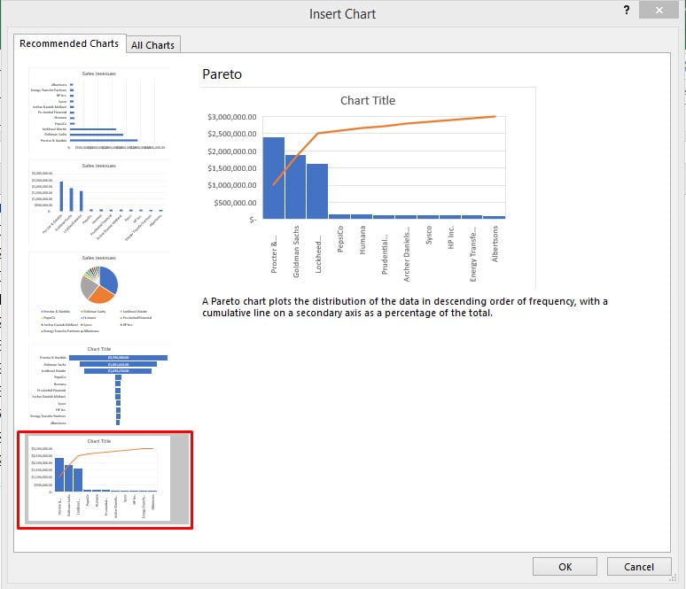
Regardless of the procedure adopted, the Pareto chart will be immediately inserted into your spreadsheet.

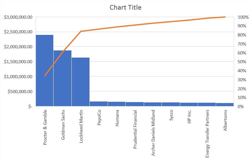
At this point, you need to add the title of the chart.

How to customize Pareto chart in Excel

You can customize the Pareto chart created in Excel to your liking.

You will be able to change colors, style, show or hide data labels, and more.

Click anywhere on the Pareto chart to bring up the Chart Tools on the ribbon. Go to the Design tab and apply the styles and colors to the chart.

Now let’s see how to add data labels to the chart.

By default, it inserted the chart without data labels. To see the values, click the Chart Elements button on the right side of the chart.

Then select the Data Labels checkbox and choose where to place the labels.

If the data is not completely legible, you can make further changes.

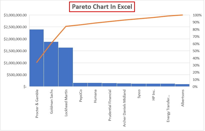
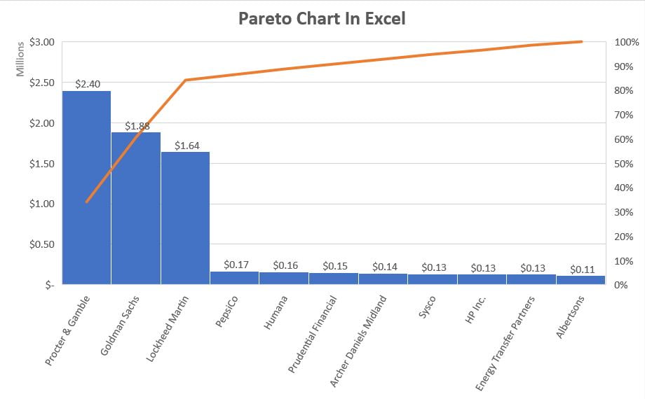
You will be able to change the display units of the graph. In the example shown, I used millions as the unit. To do this, edit the axis options from the Format Axis pane.

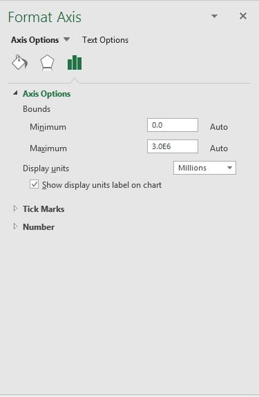
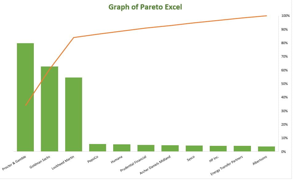
The resulting graph will look like this.

The procedure shown so far is valid if you have a version of Excel 2016 or 2019.

If your version of Excel is 2013, creating the Pareto chart will take a few more steps. Excel doesn’t have a default option, so you need to use the Combined chart type.

Finally, if you have a version of Excel 2010 or 2007, you will not have the Combined chart available.

This doesn’t mean you won’t be able to create a Pareto chart – it will take more steps and a little more work.