Statistics made easy: Microsoft Excel offers you a function for the automatic calculation of the arithmetic mean – also called “mean” or “average“. To calculate the mean on Excel, the number of values add and then divide all values. In Excel, you can either enter individual values or select cells. In this article, I want to show you a couple of really practical methods on how to find mean on excel and how it works.
How Microsoft Excel Calculates mean on Excel.
The average is basically a value calculated within a set of numbers, which, in mathematics, is known as the arithmetic mean or mean. To calculate it, what we do is add the values and divide them by the total number of numbers.
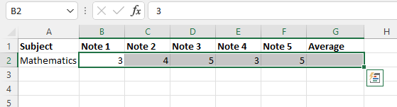
For example: let’s assume that we have the grades of any subject, in which we have got the following results (3, 4, 5, 3, 5) and we want to calculate the average obtained in that subject. Therefore, to get our average we would do it as follows, first- we add the values (3 + 4 + 5 + 3 + 5) and divide by the number of numbers (5).
The average of the marks obtained will be (3 + 4 + 5 + 3 + 5) / 5 = 4
This method is undoubtedly good, but the convenience of its use is significantly limited by the volume of processed data because it will take a lot of time to enumerate all the numbers or coordinates of cells in a large array, in this case, we can follow the procedure below to find the average on Excel.
Now, to calculate the average on Excel, we don’t have to perform all that operation, we just have to call the AVERAGE function.
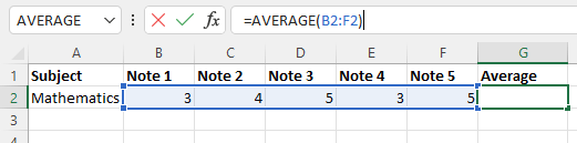
To apply the average function in Excel, select an empty cell to enter the mean formula and start the formula with an equal (=), then we write AVERAGE and select the range of which we want to calculate the mean.
= AVERAGE (B2: F2)
Find mean on Excel from Ribbon Tools
This method is based on the use of a special tool on the program tape.
1 Select the range of cells with numeric data for which we want to determine the average value.
2 Go to the “Home” tab. Find the AutoSum icon in the Editing Tools section and click on the small down arrow next to it. In the list that opens, click on the “Average” option.
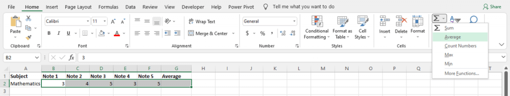
3 Immediately below the selected range, the result will be displayed, which is the average value for all the selected cells.
4 If we go to the cell with the result, then in the formula bar we will see which function was used for calculations – this is the AVERAGE operator, the arguments of which is the range of cells we have selected.
An alternative way to find mean (average) on Excel.
Go to the first free cell after the column or row (depending on the data structure) and press the keyboard shortcut “Alt+MUA” for calculating the average.
Using the AVERAGE function
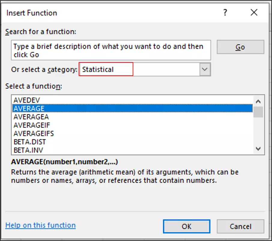
1 We stand in the cell where we want to display the result. Click on the “Insert Function” (fx) icon to the left of the formula bar.
2 In the opened window of the Function Wizard, select the “Statistical” category, in the proposed list, click on the “AVERAGE“, and then click OK.
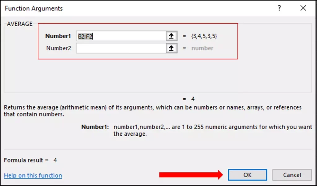
3 A window with function arguments will be displayed on the screen (their maximum number is 255). Mark the coordinates of the required range as the value of the “Number1” argument. This can be done manually by typing the addresses of the cells from the keyboard.
Alternatively, you can first click inside the field to enter information and then use the left mouse button to select the required range on the sheet. If necessary (if you need to mark cells and ranges of cells elsewhere in the sheet), proceed to fill in the “Number2” argument, and so on. When ready, click OK.
4 We get the result in the selected cell.
Tools in the Formulas tab
Excel has a special tab responsible for working with formulas. In the case of calculating the average, it can also come in handy.
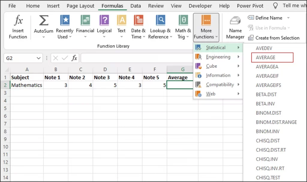
1 We select the cell in which we want to perform calculations. Go to the “Formulas” tab. In the “Functions Library” section of the tools, click on the “More Functions” icon, in the list that opens, select the “Statistical” group, then – “AVERAGE“.
2 The already familiar window of arguments for the selected function will open. Fill in the data and click the OK button.
Calculate average with a condition (AVERAGEIF)
Through the Excel spreadsheet, we can also calculate the average according to a given condition or criterion. We can do this through the AVERAGE function.
The AVERAGEIF function helps us find the average (arithmetic mean) of the cells that meet a certain condition.
AVERAGEIF function syntax
AVERAGEIF (range, criterion, [average_range])
- Range: It is the range of cells where the criteria will be searched.
- Criterion: It is the condition or criteria as a number, expression, or text that determines which cells will find the average.
- Average_range: These are the cells that will find the average. If omitted, the cells in the range will calculate the average.
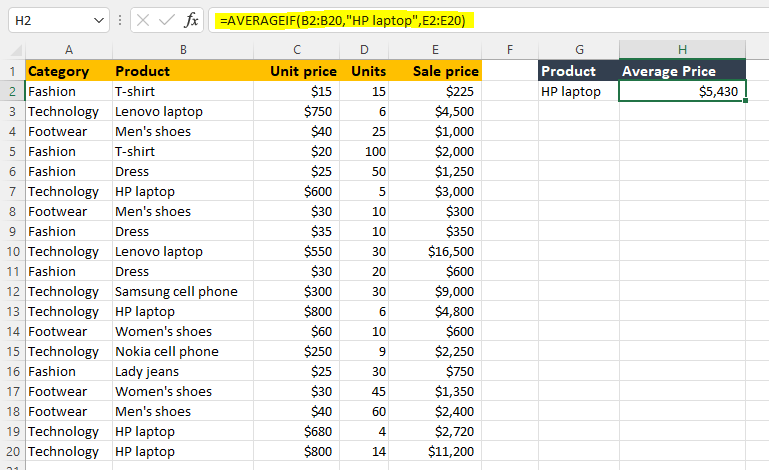
Example: We need to get the average sale price of the HP laptop product in the technology category.
To calculate the average sale price of the portable product we are going to use the AVERAGEIF function and we are going to start our formula with the equal sign (=), then we are going to choose the range where our criterion is, which for our example is in B2: B20 and the criterion or condition of our formula, located in quotation marks is “HP laptop“. Finally, we choose the range of values where the average will be applied if it meets the criteria that we have established.
= AVERAGEIF (B2: B20, “HP laptop”, E2: E20)
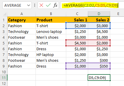
Calculate the average of numbers in non-contiguous cells
In this example, We need to get the average sale price of Sales 1 and Sales 2 in the fashion category.
=AVERAGE(C2:D2,C5:D5,C9:D9)
- So select the cell that will display the result.
- Insert Average function and select cell range C2:D2 and type comma.
- Then select the other cells range C5:D5, C9:D9.
- Close the parenthesis and validate.