Subtraction is one of the most basic things that we learned in elementary school. Similarly, Excel’s number subtraction is an easy task, and subtracting time is also an easy task.
Let’s say that you work on your own multiple projects, and want to know how much time you spent on each project. Microsoft Excel offers you various ways to calculate time in Excel. In this guide, you will find the various formula for subtracting time in Excel.
To find the elapsed time (difference between two times), follow these procedures.
Formula for subtracting time in Excel between two times to get the time difference
To determine the spending time, we frequently need to calculate the difference time between cells. There are several ways or formulas for subtracting time in Excel that we are going to discuss below.
Formula 1: Subtracting time with a simple formula
You can use a simple formula to subtract time between two-time cells.
Follow these procedures
Formula
=(End Time-Start Time)
Firstly, select the result cell (C2) and then type the formula:
=(B2-A2)
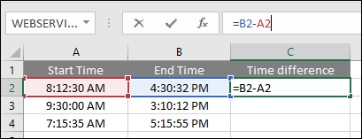
And then press Enter to see the result.
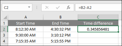
You probably know that in the internal Excel system, excel stores times in the format of a decimal number (that’s our result). So here we need to change the time formatting to display the spending times as hours, minutes & seconds properly.
1. For that purpose, select the result cell of the decimal numbers (C2 for our example) then right-click the cell and select the Format Cells in the context menu. Or press the key shortcut Ctrl+1, a Format Cells dialog box will appear.
2. In the dialog box, select the type of time format under the Time category then click OK.
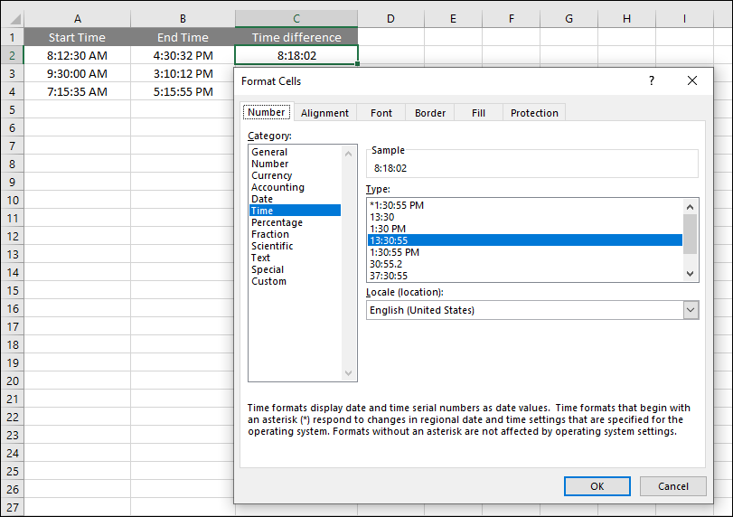
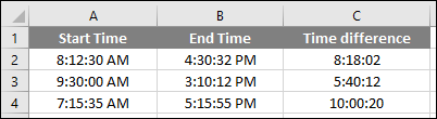
3. The decimal numbers cell has changed as hours, minutes & seconds.
4. And finally, use the Fill Handle to see the results in all the expected cells.
Formula 2: Subtracting time with the TEXT Function
You can subtract time between two times in Excel using the TEXT Function. Normally, the Text Function converts any numbers into the text string within a worksheet with one of the following formats.
| Time Format | Result |
|---|---|
| h | Display only hours (such as 3). |
| h:mm | Display hours and minutes (such as 3:20). |
| h:mm:ss | Display hours, minutes, and seconds (such as 3:20:50). |
Syntax
TEXT(value, format _ text)
Generic formula
=TEXT(End Date – Start Date, Format)
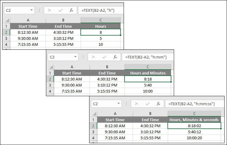
- To subtract only hours between two times: =TEXT(B2-A2, “h”)
- To subtract hours and minutes between two times: =TEXT(B2-A2, “h:mm”)
- To subtract hours, minutes, and seconds between two times: =TEXT(B2-A2, “h:mm:ss”)
Noto
TEXT formula displays the #VALUE! error, if the result is shown as a negative number.
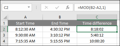
Formula 3: Subtracting time with the MOD Function
You can use the MOD function to subtract time between the two times in Excel. The MOD function basically helps us to find the remainder after dividing a number (dividend) by another number (divisor).
Syntax
=MOD(number,divisor)
Generic formula
=MOD(End Date – Start Date,1)
Select the result cell (C2) first and then type the formula
=MOD((B2-A2),1))
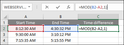
And then press Enter to see the result.
Here again, need to change the Time Format.
Finally, use the Fill Handle to see the results in all the expected cells.
Formula 4. Subtracting time in hours, minutes, or seconds
When you subtract time, Excel gives a decimal number that represents the time subtraction.
Since each integer represents a day, the decimal part represents a fraction of a day that can easily be converted into hours, minutes, or seconds.
You can use the following calculations to get the subtracting time in a single time unit (hours, minutes, or seconds).
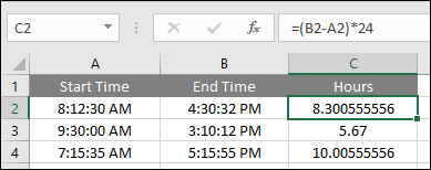
Subtracting Hours between two times
To subtract hours between two times, use this formula:
=(End time – Start time) * 24
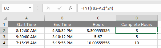
Use the INT function to round the value down to the closest integer to get the number of complete hours:
=INT((B2-A2) * 24)
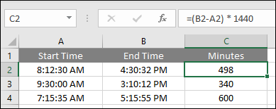
Subtracting Minutes between two times
To subtract minutes between two times, use this formula:
=(End time – Start time) * 1440
To get only minutes unit between two times, multiply the time difference by 1440, that’s the number of minutes in a day (24 hours * 60 minutes = 1440).
=(B2-A2) * 1440
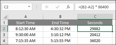
Subtracting Seconds between two times
To subtract seconds between two times, use this formula:
=(End time – Start time) * 86400
To get only seconds unit between two times, multiply the time difference by 86400, that’s the number of seconds in a day (24 hours * 60 minutes * 60 seconds = 86400).
=(B2-A2) * 86400
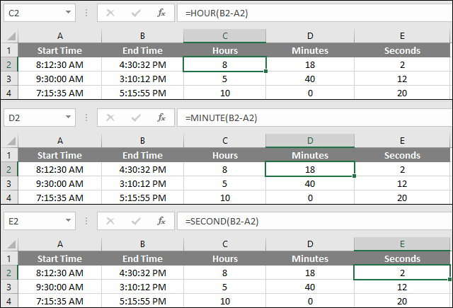
Formula 5. Subtracting time into one unit (hours, minutes, or seconds) ignoring others
Use one of the following functions to find the subtraction between two times in a specific time unit ignoring others.
| Calculation | Formula |
|---|---|
| Hours | =HOUR(B2-A2) |
| Minutes | =MINUTE(B2-A2) |
| Seconds | =SECOND(B2-A2) |
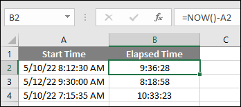
Formula 6. Subtracting time from the start to now to get the Elapsed Time
Another simple formula to subtract elapsed time from the start to now is the NOW function which returns the current date and time from the start time.
Formula
=NOW()-A2
In this example, Column B returns the following results because we’ve applied the 13:30:55 time format.
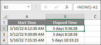
Our result shows only time because of using the 13:30:55 time format, using the d “days” h:mm:ss like in the following screenshot to get the result with the days.
Formula 7: Subtracting time with the IF Function
IF Function can also be used to subtract time between two-time cells. If the logic is correct, the IF Function returns a value. Otherwise, it will return a different value.
If start and end times span midnight, then you need to adjust by the IF Function that’s explained below.
You probably know the end time is actually less than the start time it returns a negative value that’s will display as hash (######) characters. The below formula will help you get time subtraction without any hash (######) or negative sign.
Generic formula
=IF(end>start, end-start, 1-start+end)
Formula
=IF(B2>A2,B2-A2,1-A2+B2)
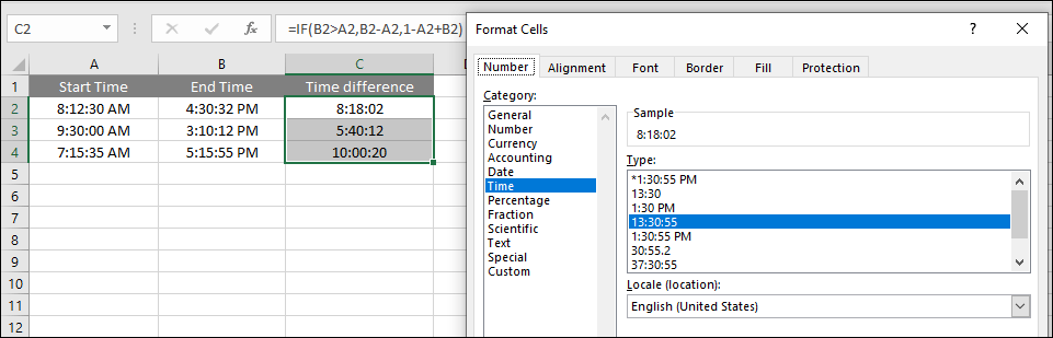
Change the Time Format, and get results in all the expected cells using the Fill Handle.
Formula 8: Display subtracting time as “XX days, XX hours, XX minutes, and XX seconds.”
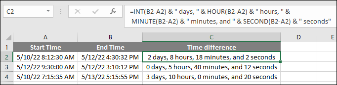
To get corresponding time units, you can use the HOUR, MINUTE, and SECOND functions, and the INT function to compute the difference in days. This formula may be most user-friendly for subtracting time in Excel between two times to get the time difference displayed as “XX days, XX hours, XX minutes, and XX seconds.”
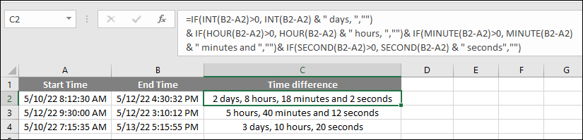
If you want to hide zero values in this subtracting time, then you can use the below formula.
=IF(INT(B2-A2)>0, INT(B2-A2) & ” days, “,””) & IF(HOUR(B2-A2)>0, HOUR(B2-A2) & ” hours, “,””) & IF(MINUTE(B2-A2)>0, MINUTE(B2-A2) & ” minutes and “,””) & IF(SECOND(B2-A2)>0, SECOND(B2-A2) & ” seconds”,””)
Results Showing Hash (###) Instead of Date/Time (Reasons + Fix)
Sometimes Excel is displaying the hash (####) symbols in our format cell when it can’t find enough space to show the result in the cell, then it can be solved by increasing column width.
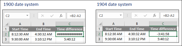
Similarly, you find the result as hash (####) in our time subtraction cells due to negative time. In this case, you can show the negative time will start showing by setting the 1904 date system.
How to change Excel date system to 1904 date system
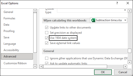
Switching to the 1904 date system is the quickest and easiest method to show negative time normally.
To do this, go to the File tab and click Options then select Advanced, scroll down to go to the When calculating this workbook section, and check the Use 1904 date system box.
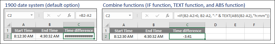
Result (1900 date system vs 1904 date system).
Combine functions so that Hash (#######) is not displayed.
Combine with the IF function, TEXT function, and ABS function to display negative times properly.
Following formula:
=IF(B2-A2>0, B2-A2, “-” & TEXT(ABS(B2-A2),”h:mm”))